Unit 2 Section 4- 6

Home

Online Grapher

Hyperglossary

Unit 2- Intercepts, Zeros, and Solutions

The second part of this chapter focuses on solving many different types of equations, both algebraically and graphically.

Graphing Calculator Skills
Section 2.4 Quadratic Equations
This section focuses on the methods of solving quadratic equations algebraically. The text uses the graphics calculator to provide the check. Check the Graphing Calculator VIDEO and manual for more information on this topic.
You should be able to solve quadratic equations by:
Factoring method, quickest if equation is easily factored.
x² + 4x + 3 = 0
(x+1)(x + 3) =0
x +1 = 0 or x + 3 =0
x = -1, -3

Square Root Principle works best when left hand side is a perfect square

(2x-3)² = 25
(2x-3) = + 5
2x = 3+ 5
x = 4, -1

Click on the logo to explore a LiveMath Notebook

Completing the square. This method is not necessarily the easiest to use, however it becomes an important method much later on in the course in the study of conic sections. It is also the method used to develop the quadratic formula.

x²+ 8x + 4 = 0
x²+ 8x = -4
Take half the coefficient of the x term and square it. Add to both sides.
x²+ 8x +16 = -4+16
(x + 4)²=12
(x + 4)= +sqrt(12)
x = -4 +sqrt(12)

Click on the logo to explore a LiveMath Notebook

Quadratic Formula This method should have been previously studied in earlier courses. It is an important method to relearn. Experiment with the following MathView worksheet to see how the values of a, b, and c affect the solutions to the general quadratic equation.

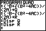
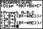
Note: Below is a program for solving quadratic equations using the TI 83 calculators.
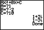
The third graphic demonstrates the progam being used.

Radical, Absolute Value, and Fractional Equations are also shown in this section along with applications. Please review the examples.
| x - 4| = 5
x - 4 = 5 or x - 4 = - 5
x = 9 or x = -1

Section 2.5 Inequalities

After solving algebraically, the easiest way to check inequalities is to use the graphics calculator. The text demonstrates many different methods for using the calculator. Please familiarize yourself with these methods. Note: the method described on the bottom of page 220 is shown below . The < , >, and = signs can be found on the TEST menu by entering 2nd MATH.

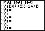
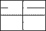
The solution is the set (-oo, -7) U (2,oo)

Section 2.6 Linear Models , Regression, and Scatter Plots.

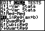
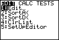
This section explains how to fit a line to data. You are only responsible to do this on the calculator. The blue section on the bottom of page 232 will help you with this, as will the video, and CD ROM. Enter data through the STAT menu. First shut off any graphs that may be on in the Y = editor. Also, to clear a list that is in the List editor from a previous problem, move the cursor up to the top of the list above the data, then press CLEAR, ENTER

Note: To turn on the regression correlation feature on the TI 83 press : 2nd, CATALOG, scroll down to DiagnosticOn, press Enter twice.

For more help on Linear regression in the TI83, please download the following file:

Example The median sale price in thousands of a new home is given by the following table.
Use linear regression to find an equation and to predict the median price in the year 2000.


Year	1986	1987	1988	1989	1990	1991	1992	1993
Price	80.3	85.6	89.3	93.1	95.5	100.3	103.7	106.8

Press STAT , Edit
Enter the Data using 6 for 1986, 7 for 1987, etc., letting year 0 = 1980.
Press STAT, CALC, 4, ENTER
On the TI 83, (see 3rd row of screens) press STAT, CALC, 4, (COMMA) then enter L1, L2, VARS YVARS, 1, 1 to have the equation pasted onto the Y-editor to make evaluation easier

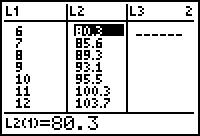
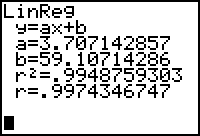
The approximate equation is y = 3.7x + 59.1. The year 2000 would be equivalent to x = 20. Either use Y1(20) or just evaluate the equation at x = 20. y = 133.1 or $133,100

To obtain the scatter plot, press 2nd STAT PLOT, ENTER. Make sure ON is highlighted, and the scatter plot is also highlighted as shown . Then press ZOOM 9.

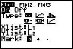
TRY it now!! Use your graphing calculator to produce the scatter plot for the above problem. You should see the plots and the graph of regession line as done above.

Click on the LiveMath logo to see the same problem explored with LiveMath.

Top

Proceed to Unit 3